General Introduction to Atomic Force Microscopy
Several of the more successful techniques used to assess the compositional quality of bone include X-Ray Diffraction (XRD), Fourier Transform Infrared (FTIR) Spectroscopy and Raman Spectroscopy. Other x-ray-based methods such as Small Angle X-Ray Scattering (SAXS) and Wide Angle X-Ray Scattering (WAXS) have been used to analyze mineral crystal thickness and larger-scale matrix organization. These techniques lack the ability to directly answer questions about the nanoscale assembly and organization of collagen and mineral in bone.
Traditional optical microscopes focus light to produce an image, and are therefore limited to a resolution of approximately 200 nm due to the diffraction limit of light (well above a true nanoscale resolution). To overcome this resolution limitation and produce images of collagen and mineral at the nanoscale, methods such as transmission electron microscopy (TEM) and scanning electron microscopy (SEM) focus electrons rather than photons. These methods can produce high-resolution images of the collagen and mineral components of the bone matrix, but both techniques have significant limitations. To perform TEM in mineralized tissues, the sample is typically fixed and fully dehydrated, embedded in a hard resin, cut with a diamond blade to produce ultra-thin sections and imaged under vacuum. For SEM, samples are dehydrated and coated with either carbon or gold to increase contrast, then imaged under vacuum. The combination of harsh sample preparation and imaging conditions may induce artifacts and ultimately reduce the accuracy of conclusions drawn from the data.
Atomic force microscopy (AFM) operates under a fundamentally different mechanism by dragging a sharpened probe over a surface and using force interactions between the surface and the probe to build a map of the sample's topography. In essence, AFM acts like a nanoscale phonograph or record player. AFM is a high-resolution imaging modality which is less-destructive than either TEM or SEM. Samples imaged using AFM can remain intact and can be imaged in air or fluid, at room temperature or under culture conditions, implying that measured properties are characteristics of the sample and less likely artifacts of processing or imaging.
A Brief History of AFM
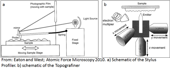
An early instrument developed by Gustav Schmalz in 1929, the stylus profile, operated by dragging a stylus mounted on the end of a rigid bar across a sample to produce a height profile. Due to bending caused as the "probe" met lateral resistance from surface features, the resolution and fidelity of the resulting image were questionable. In 1955, Becker oscillated his probe to reduce surface drag. Then in 1972, Russell Young developed the Topografiner. Young took advantage of piezoelectric ceramic materials which expand and contract in a highly controlled manner with an applied electric potential. A metal probe was mounted onto a piezoelectric element which moved the probe in the vertical direction to control the separation distance. An electron field which varied as a function of distance between the sample and probe developed. A feedback system was used to monitor the electron field and keep this distance at a constant value as the probe was scanned across a surface.
The limiting factor governing resolution of the Topografiner was vibration. In 1982 at IBM, Binnig and Rohrer finally addressed the vibration issue with the invention of the Scanning Tunneling Microscope (STM). By improving vibration isolation, they were able to monitor electron tunneling rather than field emissions. Tunneling current is more sensitive to tip-sample interactions, so the probe could be kept very close to the surface. The result was a small device that produced atomic resolution images, a feat that earned Binnig and Rohrer the Nobel Prize in Physics in 1986. Recognizing that STM was limited to electrically-conductive materials, Binnig et al. replaced the conductive wire probe with a diamond glued to a strip of gold, producing the first Atomic Force Microscope in 1986.
Basic AFM operation
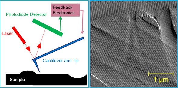
The operation of AFM for is governed by three basic components. Piezoelectric elements are used to accurately move the AFM probe in three dimensions, independently. As the probe is scanned across the sample in the x-y direction, the force of the interaction between the sample and the probe is measured by the cantilever on which the probe is mounted. A control system is used to maintain a desired force between the probe and the sample. When the measured force it larger or smaller than this set point, a voltage is applied to the z-piezo to move the probe away from or towards the surface, bringing the force back to the set point.
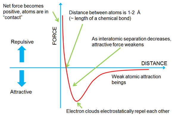
To understand AFM operation, one must recognize that interactions are occurring between the probe and sample at the molecular level. Although other forces are active, van der Waals forces typically dominate at small distances. When two objects which are initially far apart are brought closer together (e.g. the AFM probe and the sample surface), weak attractive interactions exist between atoms at the surface of the sample and those at the apex of the probe. With decreased separation distance, this attractive force increases until electron clouds begin to interact and electrostatically repel each other. This repulsive force weakens the overall attraction until a net force of zero is reached. At this point, the distance between atoms is on the order of 2-3 angstroms. Eventually, the interactive forces become positive (repulsive) and the atoms are said to be in "contact." In the "contact" region, the slope of the curve is steep meaning that the van der Waals forces balance most attempts to push the atoms closer together. In the case of AFM, when the cantilever pushes the probe against the sample, the cantilever instead deflects like a linear spring according to Hooke's law (i.e. F = -kx where k is the spring constant and x is the deflection). In essence, the cantilever is a sensitive force transducer.
AFM-based Imaging
AFM is generally operated using one of two main feedback modes. In Contact Mode, operation is in the repulsive regime and the probe remains in contact with the surface at all times. The cantilever deflects up or down to accommodate topography under the probe while a user-defined deflection (i.e. imaging force) is maintained by moving the sample using the Z-piezoelectric actuator. This Z-piezo movement at each pixel location generates a height profile image of the surface. This method of operation is good for wet or dry imaging and can approach atomic resolution. A limitation is that constant contact with the surface can cause damage to both the sample (especially soft samples) and the probe as lateral forces develop with scanning.
In Intermittent Contact or Tapping Mode, the cantilever is oscillated near its resonance frequency (in the 10's to 100's of kHz) as the probe is scanned across the surface. The amplitude of oscillation is typically set between 10 and 100 nm, and the probe "taps" the surface at the bottom of its bounce. As the probe interacts with topographic features, the oscillation amplitude changes and the feedback loop moves the sample up or down to maintain the amplitude set point. Since the probe is in contact with the surface for a fraction of its tapping period, lateral forces are reduced. A drawback of this method is that imaging in fluid can be challenging. The cantilever must be "tuned" at its resonance frequency, which is straightforward in air but in fluid, the resonance frequency is often altered and spurious peaks exist.
PeakForce Tapping is a recently implemented imaging mode which oscillates the probe at a set frequency of 1 kHz. Because of this relatively slow tapping rate, a force curve can be generated with each tap and the maximum (peak) force of the tap is used as the feedback signal. Because force is directly controlled, it can be minimized to reduce sample damage and tip wear. In addition, because the cantilever is not tuned, imaging in fluid is much less challenging.
AFM-based Indentation
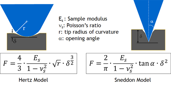
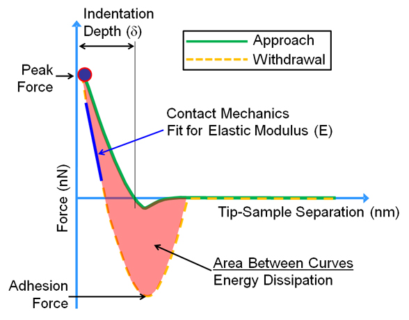
Since the cantilever is a sensitive force transducer, the cantilever/probe combination can be used to push on a sample to extract elastic mechanical properties. The probe is indented to a known load or displacement, and a force-displacement curve is collected and analyzed. Maximum (peak) force, deformation, adhesion force and energy dissipation can be found directly from the raw data. Elastic modulus (i.e. sample stiffness) is obtained from the slope of the withdrawal portion of the force curve using one of many contact mechanics approaches. The Hertz model describes the indentation of an infinitely hard spherical indenter (the probe tip) on an elastic cylinder (the sample).This model is appropriate when the indentation depth is significantly less than the radius of curvature of the probe. The Hertz model does not take adhesion into account and is often modified using the Derjaguin-Muller-Toporov (DMT) model. When the indentation depth is close to or exceeds the radius of curvature of the probe, the Sneddon model of contact between an infinitely hard conical indenter and an elastic cylinder is more appropriate. A major strength of AFM-based indentations is that it is a true nanoscale approach, where the forces and deformations remain "nano" in scale. In a traditional "nano"indentation test, forces of greater than 1 mN are not uncommon, leading to large deformations on the order of 1 micron. This level of indentation force can lead to local yielding and permanent deformation of the sample.